results <- read.csv("data/experiment.csv", header = TRUE)
head(results)
group time
1 none 1241
2 none 1215
3 mild 1060
4 mild 1084
5 strong 1005
6 strong 1005In this chapter, we explain one of the fundamental research methods, controlled experiments. A controlled experiment is typically used to answer research questions in the form “Does X cause Y?” or “Is A more efficient/precise than B?”.
Suppose we would like to know what is the relation between playing platform games and kids’ typing speed on a computer keyboard. We start asking a very large random sample of kids whether they are playing platform games. During the study, we also measure the typing speed of each participant using a standardized test. As a result, data similar to Table 5.1 is produced, with hundreds of rows.
| Participant ID | Plays platform games | Typing speed (words/min) |
|---|---|---|
| 1 | false | 32 |
| 2 | false | 21 |
| 3 | false | 25 |
| 4 | true | 65 |
| 5 | true | 53 |
| 6 | true | 67 |
| … | … | … |
For all participants not playing platform games, the mean is 27 words per minute, while for the playing ones, a mean of 62 was computed. Platform game players thus seem to be markedly faster at typing. Suppose we report our findings in a research paper that gets published. After some time, a famous tabloid comes with a flashy headline:
“Playing platform games improves typing speed” say researchers.
Based on this fantastic news, many parents sign their kids up for a platform gaming club. Every week, they play Super Mario, Crash Bandicoot, Seiklus, and other popular platformers. Sadly, after a year of playing, the parents find out there is absolutely no difference in their kids’ typing speed.
Why is this the case? Clearly, there is a difference between correlation and causation. The study showed there is a correlation: “Kids who play platform games tend to type faster”. However, it did not show causation at all: “Playing platform games causes kids to type faster.”
The question arises about what is the true causation in our example. Is it reversed, i.e., typing faster causes kids to play computer games? In general, reverse causality is possible, but in our specific example, this does not seem plausible. Instead, we should look at other hidden variables that were not measured in our study. During interviews with the participants, we might find out that practically all kids that play platform games also chat using various instant messaging applications. In Table 5.2, there is a new column “chats”, representing a confounding factor, which is a variable related both to the incorrectly presumed cause (playing platform games) and the outcome (typing speed).
| Participant ID | Plays platform games | Chats | Typing speed (words/min) |
|---|---|---|---|
| 1 | false | false | 32 |
| 2 | false | false | 21 |
| 3 | false | false | 25 |
| 4 | true | true | 65 |
| 5 | true | true | 53 |
| 6 | true | true | 67 |
| … | … | … | … |
Upon closer investigation, we might find that the reality is even more complicated, as the root cause of both game-playing and chatting is that a given kid has a dedicated computer at home. This situation is displayed in Figure 5.1.

In general, there may be many confounding factors. We could carefully search for such confounding factors and take them into account during statistical calculations. This process is called controlling for variables. However, if practically possible, a much more valid approach should be applied instead: a controlled experiment.
A controlled experiment is based on the idea that we keep all conditions fixed, while manipulating only the presumed cause. In a very common type of a controlled experiment, a randomized controlled trial, we randomly divide a set of subjects (e.g., people, programs) into two or more groups. Each group receives a different treatment; if a group receives no treatment at all (or a placebo), it is called a control group. At a specified time(s), we measure the outcome for each subject and compare the results between the groups. This approach works, particularly with a large enough number of subjects, because randomization diffuses the subjects having various characteristics into all groups.
In our example, we could divide the kids (preferably the ones not playing platform games regularly) randomly into two groups. The first one will play platform games for two hours a week, while the second one will not play platform games at all. After a few months, we compare the typing speed of the groups.
Before performing a controlled experiment, we need to define variables. A variable in research is a measurable, observable, or manipulable characteristic that can vary. An independent variable is a condition which we manipulate in the controlled experiment. A dependent variable is an outcome which we measure or observe. Its name is derived from the fact that we hypothesize it depends on the value of the independent variable. In some cases, a mediating variable, influenced by the independent variable and affecting the dependent variable, can stand between these two variables and explain the relationship.
Each variable has a scale. There are four possible scales:
The list is ordered from the most general scale to the most specific one, so if an appropriate statistical test exists only for a more general scale, it can be applied instead.
In our example experiment, an independent variable of a nominal scale is playing/not playing platform games. A dependent variable of a ratio scale is the typing speed in words per minute.
Next, we define a null and alternative hypothesis. A null hypothesis, denoted H0, assumes there will be no difference between the groups in the experiment, which means changing the value of the independent variable does not cause a change of the dependent variable. An alternative hypothesis (H1 or Ha) stipulates a difference between the groups will be present, so there is a causal relationship between the independent and dependent variable.
In our example, the null and alternative hypotheses could be defined as follows:
The alternative hypothesis in our example is a two-tailed hypothesis since it considers a change in both directions; the difference could be either positive or negative. A one-tailed hypothesis would consider only the specified direction and deny the possibility of the opposite one, e.g., “Playing platform games improves the typing speed of kids.” We should generally use a two-tailed hypothesis unless we have good reasons not to do so, such as when the opposite change is impossible or irrelevant.
An experimental design formally defines how the experiment will be executed. It tells us how the assignment of the subjects to groups will be performed. It also specifies how many times and in what order the treatment will be administered and the outcome measured.
Based on the randomness of the assignment of the treatments to the subjects, we distinguish:
From the perspective of the sequence of treatment administration and measurement events, there exist multiple experimental designs. The most common ones are:
Another categorization specifies the number of treatments each subject receives. In a between-subject design, each subject is assigned to one specific group during the whole experiment, receiving only one treatment. Table 5.3 shows an example of such a design.
| Subject ID | Treatment |
|---|---|
| 1 | 1 |
| 3 | 1 |
| 5 | 1 |
| … | … |
| Subject ID | Treatment |
|---|---|
| 2 | 2 |
| 4 | 2 |
| 6 | 2 |
| … | … |
When using a within-subject design, each subject receives a treatment, and then the outcome is measured. Then the same subject receives another treatment, and the outcome is measured again. If there are more treatments, these steps are repeated. Table 5.4 displays an example of the assignment of the subjects to treatments in a within-subject design with two treatments. Note that we used counterbalancing, i.e., subject #1 was administered treatment 1 first and then treatment 2, while subject 2 received them in the reversed order. This is done to prevent systematic bias, where one of the treatments would be given an advantage.
| Subject ID | First treatment | Second treatment |
|---|---|---|
| 1 | 1 | 2 |
| 2 | 2 | 1 |
| 3 | 1 | 2 |
| 4 | 2 | 1 |
| … | … | … |
A between-subject design is usable in almost all situations, but it requires more subjects than the within-subject design. On the other hand, a within-subject design requires fewer subjects, but the learning effect and fatigue are a problem when the subjects are human.
An experiment can have multiple independent variables. The most straightforward way is to have a group for every possible combination of independent variables. For instance, with two dichotomous variables, we would have four groups. This is called a factorial design.
Suppose we execute our example experiment and collect the data. Let us say the mean of the not-playing group in the controlled experiment is 45.1 words/minute, and the mean of the playing group is 45.8. Therefore, we can say that on average, the playing group was 0.7 words/minute – or 1.6% – faster. These are one of the simplest ways to express the effect size. Although they are valid and easily comprehensible, there exist standardized metrics of effect sizes, such as Cohen’s d, which take variability (standard deviation) into account and simplify the meta-analysis of multiple papers. Kampenes et al. (2007) provide a systematic review of effect sizes commonly used in software engineering, including an overview of the possibilities.
One question remains: Are these two mean values (45.1 and 45.8) sufficient to reject the null hypothesis (no difference) and accept the alternative hypothesis? The answer is no because the difference in means could be observed purely by chance. We need to analyze the whole dataset to find whether the result is statistically significant.
For this, we compute a p-value, which is the probability of observing the data at least as extreme as we observed if H0 was in fact true. The largest acceptable p-value is called a significance level, denoted \(\alpha\), and must be stated before the execution of the experiment. The most commonly used value of alpha is 0.05 (i.e., 5%). If \(p < \alpha\), we reject the null hypothesis, otherwise we fail to reject it.
The p-value is computed by an appropriate statistical test. To select a test, we can use, e.g., a table by UCLA or by Philipp Probst. Each test should be applied only in situations when its assumptions are met. For instance, the independent-samples t-test has multiple assumptions: the data should be approximately normally distributed, there should be no significant outliers, etc. Many statistical tests are implemented in the libraries of programming languages, such as R or Python.
Let us say that in our example, the computed p-value would be 0.67. This means we could not reject the null hypothesis, so we would not show there is any effect of playing platform games on typing speed. If the p-value was, for instance, 0.04, we would reject the null hypothesis and show an effect.
In Table 5.5, we plotted the computed result of the experiment (rejection of H0 or a failure to do so) against the reality, which is unknown. Correctly rejecting or not rejecting H0 is called a true positive and a true negative, respectively. Accepting the alternative hypothesis, i.e., showing an effect, while there is in fact no effect, is called a Type I error. The maximum acceptable probability of a Type I error is \(\alpha\), as we already mentioned.
| In reality, H0 is | |||
|---|---|---|---|
| true (no effect) | false (effect) | ||
| We reject H0 | no | true negative | Type II error |
| yes | Type I error | true positive | |
There is also another type of error in Table 5.5: a Type II error. It means we failed to show an effect when there actually is one. The probability of a Type II error is denoted \(\beta\) (beta), with a common value of 0.2. To mitigate a Type II error, we should perform the experiment with a large enough number of subjects and choose a suitable statistical test, so the experiment will have enough power (\(1 - \beta\)). It is possible to estimate the number of subjects required for a given statistical test to have the given power using a process called power analysis.
Every research project has issues that could negatively affect its validity, which we should mention in the report in a section called “Threats to Validity”. In controlled experiments, these are some common types of validity which can be threatened:
In addition to listing the validity threats, we should also mention how we tried to mitigate them or why it was not possible.
To show the whole picture, now we will describe a complete example of an imaginary controlled experiment, along with the data analysis using the R statistical programming language. Suppose we have the following research question (RQ): Does the syntax highlighting type (none, mild, strong) affect the developers’ speed when locating a code fragment?
We formulate the null and alternative hypothesis:
We will test with \(\alpha\) = 0.05.
There is one independent variable: syntax highlighting type. It is nominal (categorical) with 3 levels. The dependent variable is of the ratio type (code location time in seconds).
One developer cannot search for the same code fragment multiple times using different highlighting styles because of a learning effect. We could use different code locations and source files for each syntax highlighting type, but different locations/files can be of varying difficulties. We also had a large pool of participants available. Therefore, we used the between-subject posttest-only design.
We recruited 33 final-year computer science Master’s students. We divided them randomly into 3 groups (none, mild, strong).
They were given 10 source code files. For each source code file, there were two tasks specified, such as: “Find the first ternary operator in the function sum()” or “Find the exception handling code in a function which receives a JSON object”.
After reading each task, the subject pressed a shortcut to display the code file. At this moment, the timer started. After finding the fragment, the participants placed a cursor on it and pressed another shortcut – if the location was correct, the timer stopped. The total time was recorded for each subject.
The measured values are located in a CSV file, of which we show only the first few rows for brevity.
results <- read.csv("data/experiment.csv", header = TRUE)
head(results) group time
1 none 1241
2 none 1215
3 mild 1060
4 mild 1084
5 strong 1005
6 strong 1005A graphical overview of the differences between groups in the form of a box plot follows.
results$group <- factor(results$group, c("none", "mild", "strong"))
boxplot(time ~ group, results)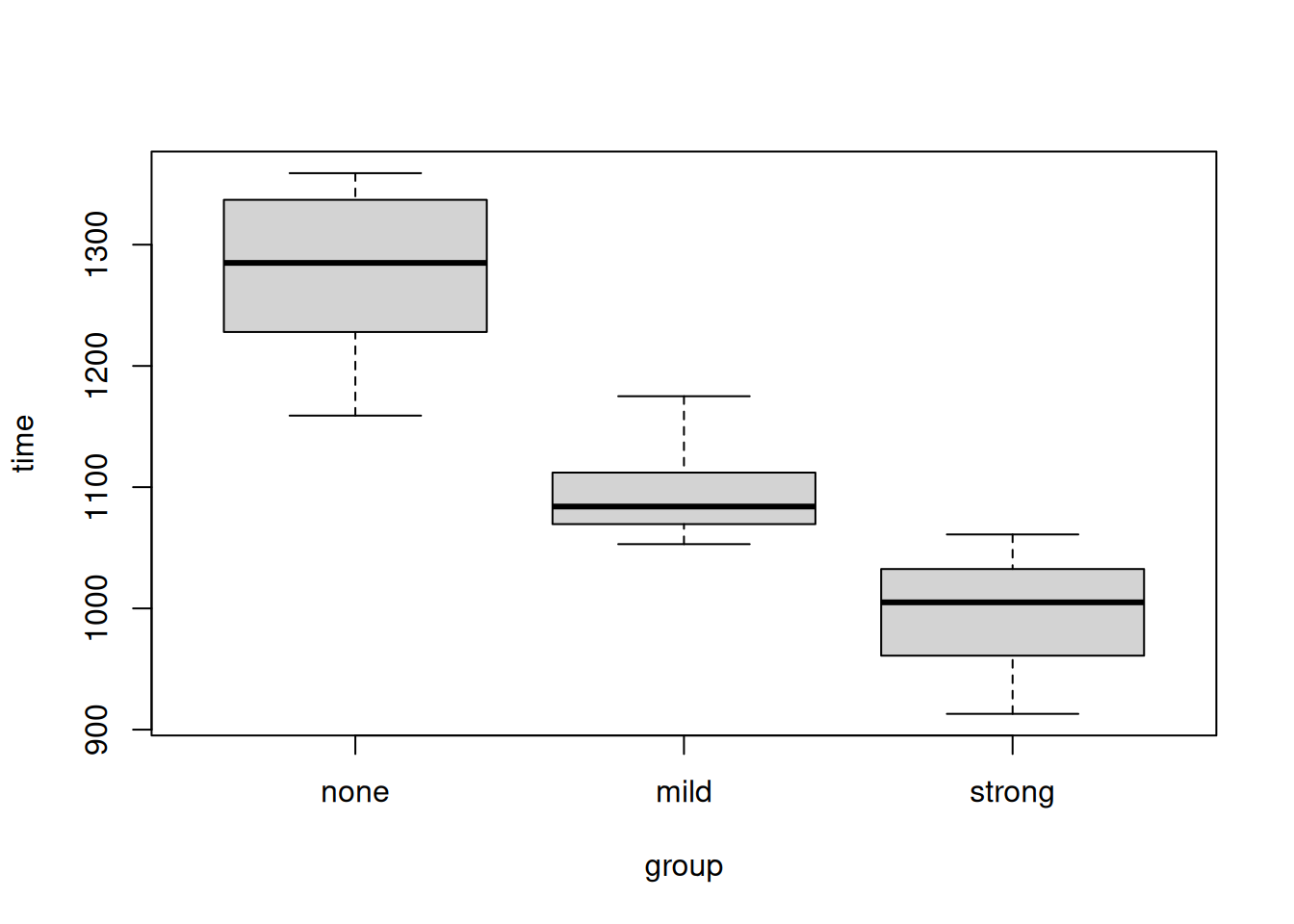
We compute the means of each group:
aggregate(time ~ group, results, mean) group time
1 none 1275.0000
2 mild 1097.0909
3 strong 993.5455How much faster were the developers (i) with mild formatting compared to none and (ii) with strong formatting compared to none?
difference <- function(col1, col2) {
    diff = (mean(results[results$group == col1, "time"])
            / mean(results[results$group == col2, "time"]))
    paste(round(100 * (1 - diff), 3), "%")
}

print(difference("mild", "none"))
[1] "13.954 %"print(difference("strong", "none"))[1] "22.075 %"To find an appropriate statistical test, we first determine whether the data are normally distributed.
options(repr.plot.width = 6, repr.plot.height = 3)
par(mfrow = c(1, 3))

for (group in levels(results$group)) {
    hist(results[results$group == group, "time"], main = group, xlab = "time")
}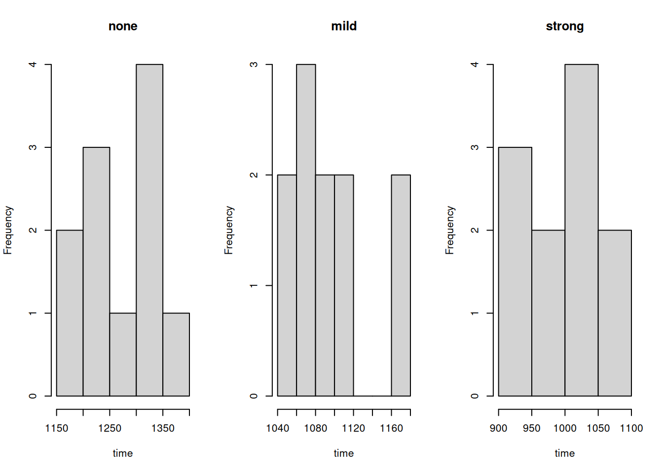
Since the data are not normally distributed, we will use the Kruskal-Wallis test.
kruskal.test(time ~ group, results)
    Kruskal-Wallis rank sum test

data:  time by group
Kruskal-Wallis chi-squared = 27.312, df = 2, p-value = 1.173e-06
Since the p-value is less than 0.05, we reject the null hypothesis. There is a statistically significant difference between the groups.
Developers performed the best using the strong highlighting type (22% faster than with none), followed by the mild highlighting (14% faster than with none). The results are statistically significant.